
Optimizing Grouped GEMM
for MoE on Blackwell
The core operation in most Mixture-of-Experts (MoE) workloads is applying each expert to all of the tokens it gets assigned. The naive way to implement this would be as a series of matrix multiplications (MatMuls): compute the output of expert 1, then expert 2, and so on. This approach has two problems:
- It suffers from many kernel launch overheads, as a new kernel is launched for each expert
- Because these multiplications are typically small relative to dense layers, these kernels potentially under occupy the GPU
As such, most implementations use a specialized Grouped GEMM kernel, which fuses all of these multiplications together, computing the outputs of all experts in parallel, with a single launch. This is also the kernel through which Pearl mining is implemented on MoE workloads. In this post, we discuss several optimizations performed by the Pearl team on grouped GEMM. The resulting kernel is faster than all other implementations we tested, and in some cases has a 15% speedup over the best-performing baseline we found (quack), mostly in small decode shapes.
Grouped GEMM
Concretely, say we have E experts W1, …, WE1, each of shape (k, n), and activations A of shape (m, k). Each of the m activations is routed to T experts so that, assuming uniformity in the routing (which is commonly encouraged during MoE training; see [1] [2]), each expert gets mT/E tokens. So we need to compute E matmuls, each, on average, of the shape (mT/E, k) @ (k, n).
To see the problems discussed in the intro play out in practice, let's plug in some numbers from the GLM 5.3 model served by Pearl. We'll assume the model is served on 8×B200 in DP=8 and EP, and a decode batch size of 512 tokens, giving m = 64 tokens per GPU. For example, for the fused MoE gate/up projection, the weights are each of shape (k=6144, n=4096).
We have E = 256/8 = 32 experts per GPU2, with each token routing to T = 8 experts. Plugging this into our formula, per GPU, we have 32 matmuls of shape (16, 6144) @ (6144, 4096). Even if we use a small tile size of (64, 64), we still have only ceil(16 / 64) * ceil(4096 / 64) = 64 CTAs, which only fills up about a third of the 148 SMs of a B2003.
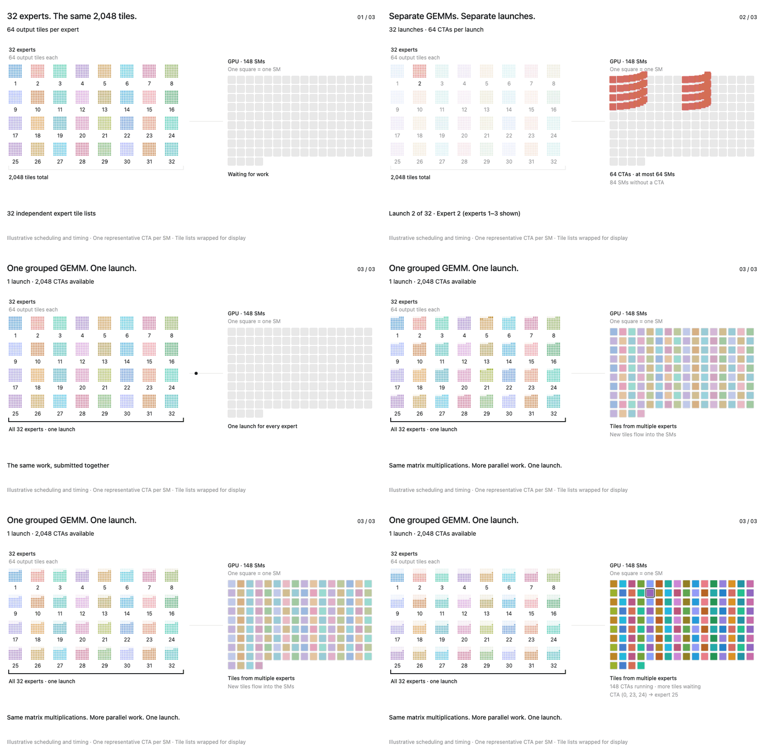
So, what do we do instead? In a regular GEMM, CTA (x, y) computes the (x, y)-th (bM, bN)-sized tile of the output matrix. Instead, in a grouped GEMM, we'll have CTA (x, y, z) compute the (x, y)-th (bM, bN)-sized tile of the z-th output matrix4. The resulting design is a tweak over a regular GEMM and quite elegant. We assume that n and k are fixed between the different GEMMs, but that m can vary. As expected, this brings us a factor 32x increase in the number of CTAs to 32*64=2048, and reduces the number of kernel launches from 32 to 1.
Below, we illustrate how grouped GEMM better utilizes the GPU.
Our Kernel
Our optimization work began by agentically porting FlashInfer's C++ kernel to CuTe DSL for faster iteration time. Then, because we saw that quack was faster from the resulting kernel, we used techniques from quack inside the kernel. Finally, we ran a day-long agentic optimization loop to find the rest of the optimizations. Below, we discuss the main optimizations it found.
Increasing # bytes in flight
Because up until a relatively large ridge point the kernel is IO-bound, loading the weights efficiently is paramount to performance. This is especially evident for small batch sizes, where because there is less activation data, the proportion of weight loading from the kernel time is much greater.
As common in GEMMs starting on Hopper, to overlap memory loads with computation, the kernel uses a pipeline while the tensor cores compute on one tile, upcoming tiles are loaded into SMEM using the TMA. Increasing the number of pipeline stages allows the kernel to have more input data in flight, but requires more SMEM. To make room for more stages, we searched for SMEM usage in the kernel, and found two places where we could reduce it.
Direct register → GMEM Store
The first was the output buffer. After computing an output tile, the kernel's epilogue stages the result through a 24KB SMEM buffer before writing it to GMEM via TMA. We found that avoiding staging through SMEM, and instead writing directly from registers to GMEM does not incur performance degradation, and allows us to eliminate this 24KB buffer.
In order to optimize these stores, we initially used STG.128 16-byte stores. However, these were not fast enough, and generated too much L2 traffic, harming performance. Instead, using STG.256 halved the number of stores, which brought us back to the SMEM-staging version's performance. The freed SMEM made room for a 7th pipeline stage, which reduced latency by about 2% at the small batch sizes.
Now, the output store looks like this:
# For each output chunk we've computed in registers
for j in cutlass.range_constexpr(cute.size(rC) // chunk):
    # If it's a valid chunk and doesn't exceed the global output's n-dimension
    if col0 + j * chunk < n:
        # Make the global tensor with alignment 32
        gC_chunk = cute.make_tensor(
            cute.make_ptr(
                self.c_dtype,
                row_base + j * chunk * elem_bytes,
                cute.AddressSpace.gmem,
                assumed_align=32,   # 32 -> STG.256, 16 -> STG.128
            ),
            cute.make_layout(chunk),
        )
        # Make the copy
        cute.autovec_copy(
            cute.make_tensor(rC.iterator + j * chunk, cute.make_layout(chunk)), gC_chunk
        )
Smaller Tile
The second opportunity was the activation tile size. To reduce shared memory usage, we tested the effects of tile_m = 64. Quack does support this, but only in 2-CTA mode, where 2 CTAs cooperate on a single output tile. Allowing this in 1-CTA as well opened another tuning region.
This reduces each activation stage from 16 KB to 8 KB, leaving more shared memory for the pipeline. In addition, using a smaller tile increases the number of CTAs, which is often also beneficial at small problem sizes, as it allows us to enjoy the benefits of wave quantization.
After adding support for 64-row tile, we noticed that our autotune system consistently selected such tiles for workloads where average number of tokens per expert is at most 64, reducing latency by 2-3%.
Increasing the size of weight loads
Previously, each B stage held one tile along the K dimension. However, optimizing SMEM usage for the activation stages as shown above let us increase this to multiple adjacent K tiles. This allows a single TMA request to fetch a wider, contiguous section of each row. This improves memory access locality while keeping enough weight data in flight to overlap the loads with computation.
This change consistently improved the smaller benchmark cases across three verification runs, reducing runtime by about 5% on each. Since the change increased both the request width and the amount of buffered weight data, the result reflects the combined effect of the two. On the producer side, things now look like this:
for k_tile in cutlass.range(0, k_tile_cnt, 1, unroll=1):
    a_stage = ab_producer_state.index                       # this entry's A stage
    tma_bar = ab_pipeline.producer_get_barrier(ab_producer_state)

    # Every other K tile opens a new B stage. That entry must own the stage
    # before its box is issued, and its barrier counts the stage's bytes too.
    opens_b = k_tile % self.b_stage_k_tiles == 0             # b_stage_k_tiles == 2
    entry_tx = a_tx                                           # bytes this entry waits for
    if opens_b:
        entry_tx = a_tx + Int32(self.num_tma_b_bytes)         # + the 32 KB B stage
    ab_pipeline.producer_acquire(ab_producer_state, peek_ab_empty_status, expected_tx=entry_tx)
    if opens_b:
        b_pipeline.producer_acquire(b_producer_state)         # a free B stage (empty-side only)

    cute.copy(tma_atom_a, tAgA_slice[(None, k_tile)], tAsA[(None, a_stage)], tma_bar_ptr=tma_bar)
    if opens_b:
        # One TMA box = two adjacent K tiles of every B row: 256 contiguous bytes
        # per row per request instead of 128.
        cute.copy(
            tma_atom_b,
            tBgB_slice[(None, k_tile // self.b_stage_k_tiles)],
            tBsB[(None, b_producer_state.index)],
            tma_bar_ptr=tma_bar,
            cache_policy=b_policy,
        )
        b_producer_state.advance()
    ab_producer_state.advance()
And on the consumer:
b_stage_idx = b_consumer_state.index
b_kblock0 = (k_tile % self.b_stage_k_tiles) * cute.size(tCrA, mode=[2])   # 0 or 4 k-blocks in
closes_b = k_tile % self.b_stage_k_tiles == self.b_stage_k_tiles - 1 or k_tile == k_tile_cnt - 1

ab_pipeline.consumer_wait(ab_consumer_state)              # A tile (and B stage, if opening) landed
for kblock_idx in cutlass.range(num_kblocks, unroll_full=True):
    cute.gemm(
        tiled_mma, tCtAcc,
        tCrA[(None, None, kblock_idx, ab_consumer_state.index)],
        tCrB[(None, None, b_kblock0 + kblock_idx, b_stage_idx)],   # this K tile's half of the stage
        tCtAcc,
    )
ab_pipeline.consumer_release(ab_consumer_state)           # A stage back to the producer
if closes_b:
    b_pipeline.consumer_release(b_consumer_state)         # B stage back, after its last K tile
Overlapping the epilogue with the next tile
At larger batch sizes, we use larger tiles (e.g. 2-CTA 256x512 ones). For such tiles, we found another source of idle time: waiting for the epilogue to release the accumulator.
Recall that the TMEM of each SM consists of 128 lanes and 512 columns, where each entry is 4 bytes. A 128-row accumulator with tile_n = 256 uses half this space, allowing for two accumulator stages, so that while the epilogue reads the result of one tile, the mainloop can start computing the next tile in the other stage.
However, with tile_n = 512, the accumulator fills the entire TMEM, leaving room for only one stage. Thus, before the mainloop can start working, it must wait for the epilogue to finish reading the entire accumulator, which takes time.
To start computing the next tile before the epilogue finishes, we make the following observation: the 512-wide tile is computed in two independent parts; for each K block, the kernel issues two 256-wide UMMA operations, one accumulating into columns 0-255, and one into 256-511. Both read from the same A/B pipeline stage, but they write into different halves in TMEM.
So, we kept the TMEM layout as is, but gave its pipeline two independently synchronized slots, one for each half. Now, the epilogue can release the first half without waiting for the second, and free up the mainloop to compute the first half of the next tile.
In the epilogue, things now look like this:
subtiles_per_slot = subtile_cnt // 2          # first 8 subtiles are atom 0, last 8 atom 1

for subtile_idx in range(subtile_cnt):
    cute.copy(tiled_copy_t2r, tTR_tAcc[subtile_idx], tTR_rAcc)   # TMEM -> registers

    if (subtile_idx + 1) % subtiles_per_slot == 0:
        # Last TMEM read of this half: hand its columns back to the MMA warp
        # now, before converting and storing. The mainloop may start writing
        # the next tile into columns 0..255 while we still read 256..511.
        cute.arch.fence_view_async_tmem_load()
        acc_pipeline.consumer_release(acc_consumer_state)
        acc_consumer_state.advance()

    ...  # scale, convert to bf16, TMA store -- unchanged
And in the mainloop:
# Slot 0 (columns 0..255) is free; slot 1 may still be draining.
for k in range(k_start):                       # k_start = half the A/B ring
    ab_pipeline.consumer_wait(ab_state)
    mma(acc[atom 0], A[k], B[k, cols 0:256])   # atom 0 only; ring entry kept, not released

acc_pipeline.producer_acquire(slot 1)          # wait until the epilogue is done with 256..511
for k in range(k_start):
    mma(acc[atom 1], A[k], B[k, cols 256:512]) # atom 1 catches up on the same held entries
    ab_pipeline.consumer_release(...)

for k in range(k_start, k_tile_cnt):           # from here on, both atoms per k-block as before
    ...
Benchmarks
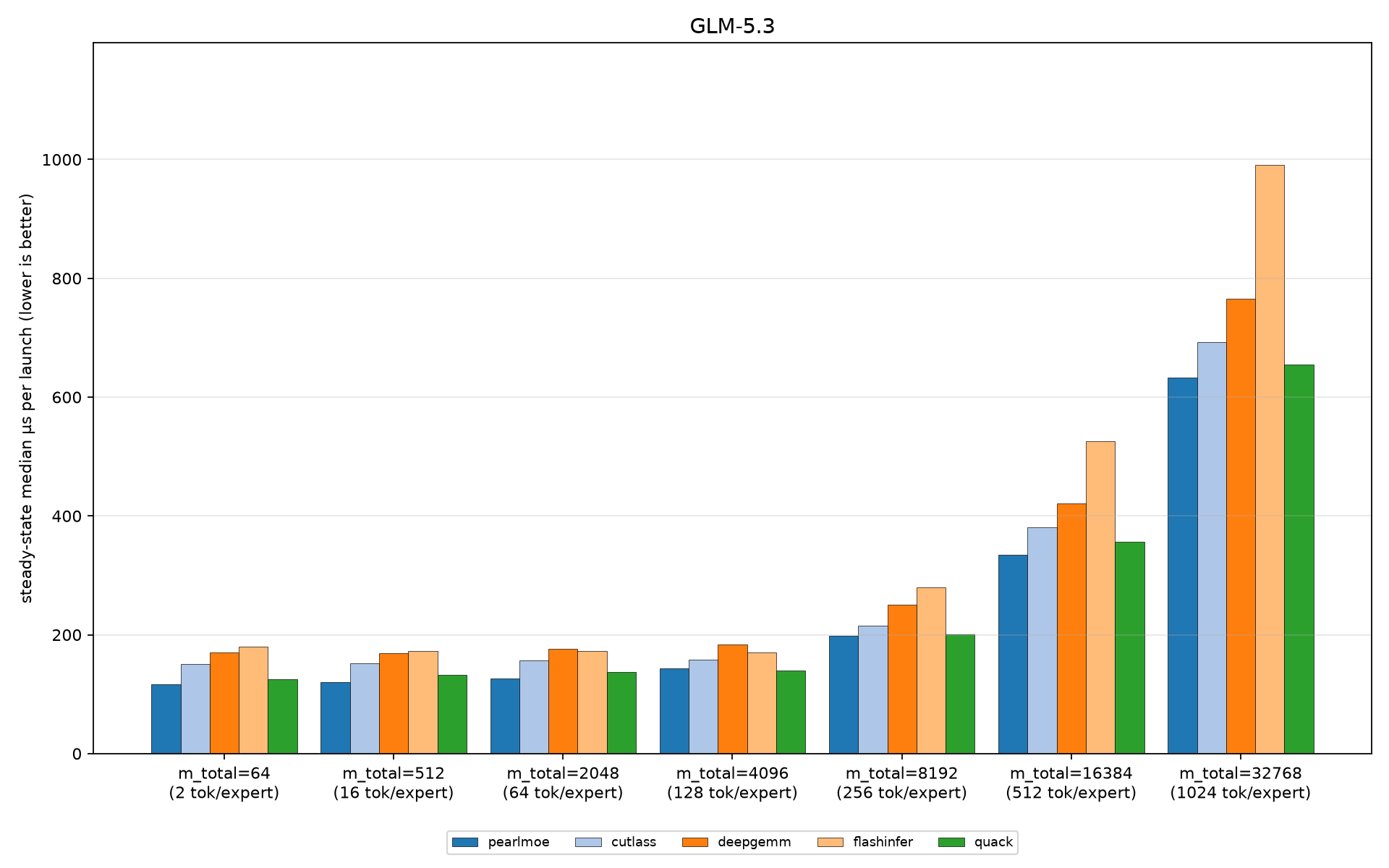
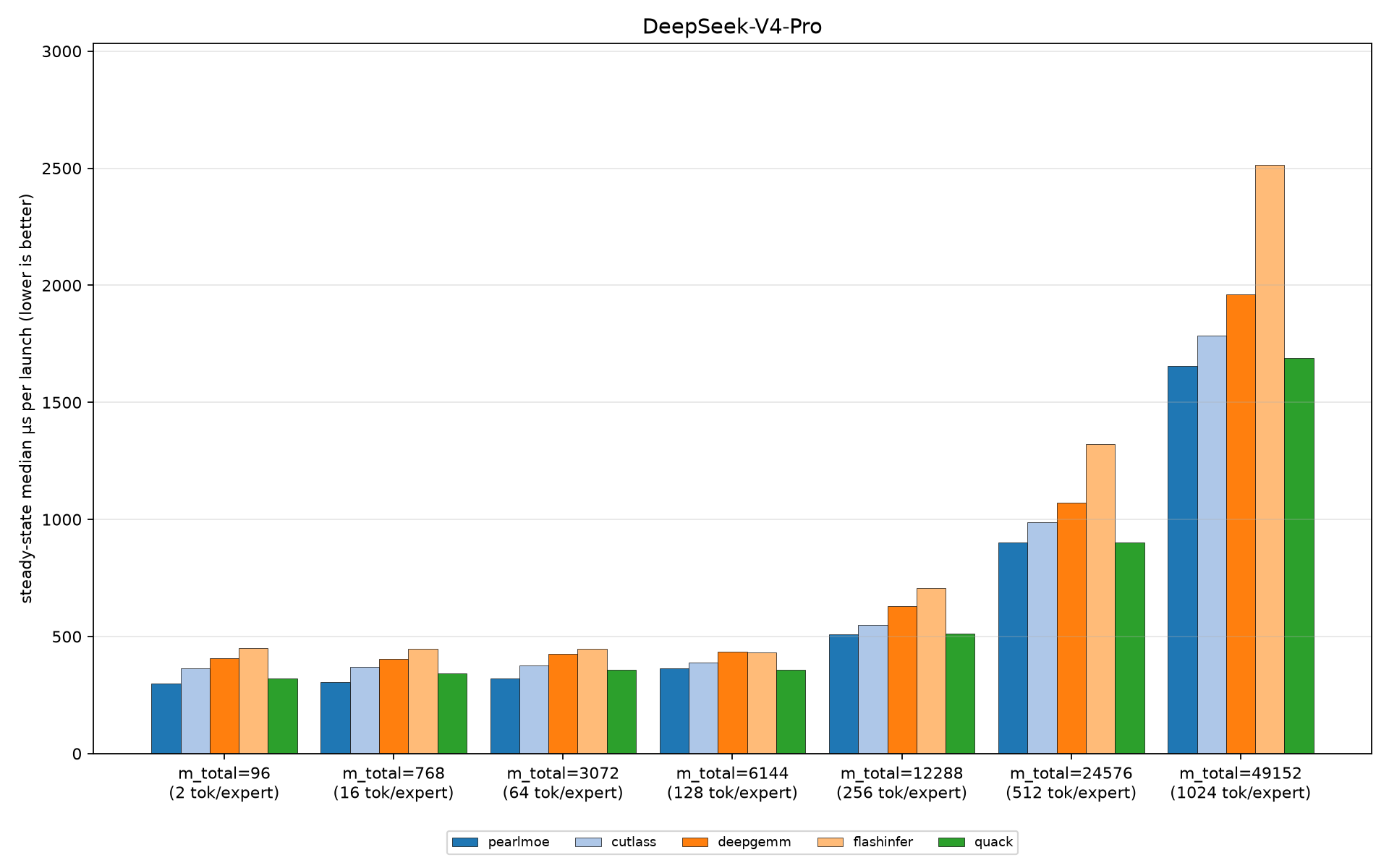
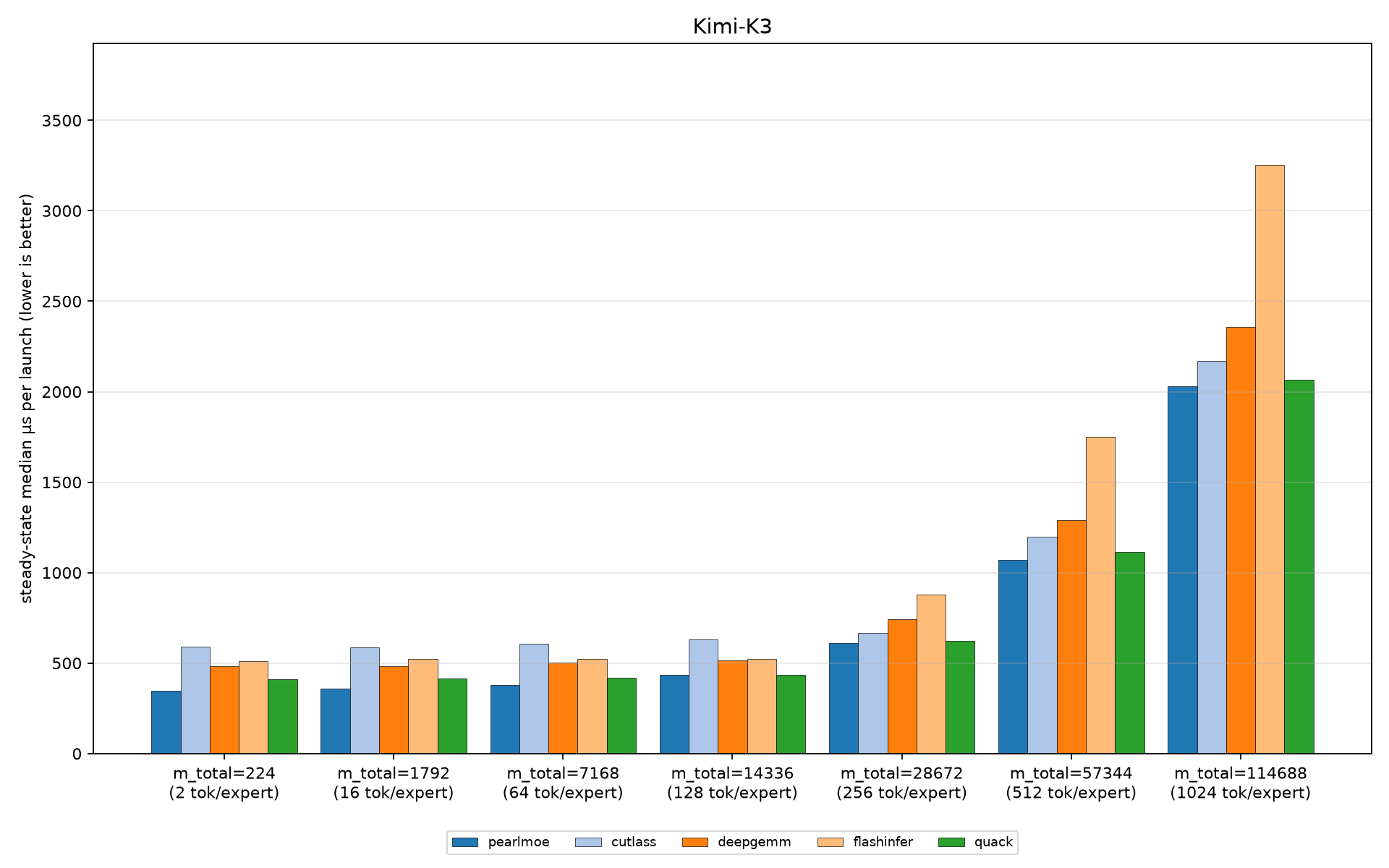
Below, we benchmark our implementation vs. other popular grouped GEMM implementations. The benchmarks are run on the gate+up shapes of the MoE layer of GLM 5.3, Deepseek v4 pro, and Kimi K3. All implementations are tuned, and benchmarked inside a CUDA graph to eliminate host overhead timing. On most of these cases, Pearl MoE outperforms all other implementations; on the losing ones Pearl MoE loses only by a small (<2%) margin. These results suggest that Pearl MoE is a promising foundation for building high-performance MoE backends.
Conclusion
In this post, we optimized the main backbone of MoE: grouped GEMM. The resulting kernel is faster than all other ones we tested, which makes it a promising foundation for new MoE backends. In the future, we also plan to enable mining inside, and optimize, MoE kernels such as Mega MoE, which fuse the entire MoE layer and multi-GPU communication into a single kernel. Such kernels present interesting alternatives to “classic” MoE backends based on a separate grouped GEMM kernel, and could also hold performance improvements.
The code for Pearl's grouped GEMM implementation will be released as part of the FP8 scheme. You can stay tuned with the latest updates on development in the development PR.
- In practice, MoE layers are usually composed of 3 “weight types”: gate, up, and down, where the first two are often fused into one matmul, and a nonlinearity (e.g., SwiGLU) is applied between gate and up. For simplicity, however, in this blog we consider MoE layers as just one type of weight. ↑
- GLM 5.3 also has a shared expert in addition to its 256 experts; like its name suggests, every token is multiplied by this expert, rather than just tokens routed to it. To keep our back-of-the-envelope calculations simple, we ignore this shared expert. ↑
- To alleviate this issue, we could, in principle, use optimizations like Split-K, but then we wouldn't be able to parallelize multiple independent GEMMs. ↑
- Depending on the kernel, a single CTA can also compute more than just a single tile, but still we get more tiles than in the serialized GEMM case. ↑