
PearlQuant: KV cache quantization
for production-scale LLM serving
TL;DR
- PearlQuant is a KV cache compression algorithm that uses high-dimensional lattice quantization, rounding groups of values together rather than each value separately, to reduce quantization error.
- Evaluated on GLM-5.3, PearlQuant uses 65% less KV cache storage per value than the FP8 baseline, with accuracy and text quality on par with FP8 in our evaluations.
- In the AgentX benchmark, replaying real Claude Code sessions on 8×B200, this configuration matches NVFP4's speed at light load. Peak throughput is 24% higher than FP8's and 22% higher than NVFP4's. At 128 concurrent sessions, it delivers 1.8× FP8's throughput.
The KV cache problem
A smaller KV cache can be the difference between waiting seconds and waiting minutes. At 128 concurrent sessions in our serving evaluation, switching from the FP8 baseline to PearlQuant cut the 90th-percentile time to first token from 144 seconds to 7 seconds. Only the KV cache quantization format changed.
Why? The KV cache stores intermediate representations of past tokens so the model can reuse them when generating new ones. As coding agents read files and accumulate tool outputs, their context grows, and so does the KV cache. On a busy server, the KV cache often becomes the bottleneck: it limits how many users a GPU can serve, and once it fills, evictions and recomputation can quickly drive up latency.
Smaller KV cache formats let each GPU serve more long-context sessions, but may hurt quality. BF16 uses 16 bits per value. Using FP8 is a common way to shrink the KV cache, and NVIDIA’s NVFP4 format [1] uses only 4.5 bits per value. KV cache quantization methods such as Google’s TurboQuant [2] target even lower rates, around 2-4 bits per value. How much can we compress the KV cache without sacrificing accuracy or speed?
Introducing PearlQuant: quantization in a high-dimensional lattice
Quantization approximates a large set of possible values with a smaller set of representative values. This set is called a codebook, and each entry is called a codeword. Instead of storing the original value, we store the index of the nearest codeword in the codebook, which requires fewer bits.
The simplest approach is scalar quantization: it rounds each number separately to the nearest codeword. PearlQuant, a NestQuant [3] based algorithm, instead uses vector quantization: it rounds groups of values together to the nearest codeword in a multidimensional codebook. For groups of d values at R bits per value, the codebook contains 2dR vectors in ℝd. PearlQuant uses groups of eight values (see the animation below).
Why eight. Quantizing values in groups reduces the error. After a random rotation, KV values behave like a Gaussian cloud: dense near the center, sparser further out. A good codebook puts its codewords where the points are dense, and gives each one a cell as round as possible (since the error is the distance from a point to its cell's center). Rounding each coordinate separately gives a rounding interval along each axis: together, these intervals form a cube-shaped cell (16 facets in eight dimensions). Quantizing eight values together lets us choose much rounder cells: PearlQuant uses the E8 lattice [4], the densest sphere packing in eight dimensions, whose cells have 240 facets. Why stop at eight? Beyond that, the gains in precision are not worth the added computational cost of quantization and dequantization.
Comparing precision per bit
PearlQuant’s rounder lattice cells give us more precision per bit. More bits mean less error, so quantization methods have to be compared at the same rate or at the same error. Information theory gives a hard limit: for Gaussian data with unit variance, the mean squared error D (the average squared difference between original and reconstructed value) cannot fall below 2−2R [5] at R bits per value (each extra bit cuts the error by 4×). Equivalently, a perfect quantizer would need at least R* = −½ log2 D bits per value to reach error D. The figure shows how many extra bits each method uses to reach the same error: its actual rate minus R*. We call these wasted bits. Zero is the theoretical limit, and lower is better. Notice that rates do not have to be integers: NVFP4, for example, stores each value in 4 bits plus an 8-bit scale shared by 16 values, averaging 4.5 bits per value.
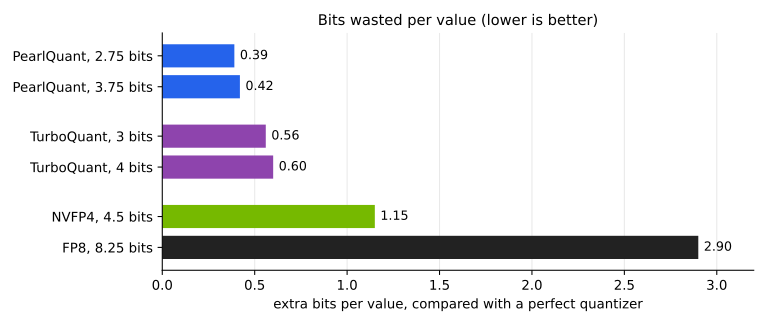
PearlQuant stays closer to the theoretical limit across all tested rates than both TurboQuant and the floating-point formats.
Figure 3 compares quantizers at uniform rates, but different components of a model’s KV cache may benefit from different rates. For example, in GLM-5.3, the FP8 baseline stores NoPE in FP8 and RoPE in BF16, averaging 9.1 bits per value. Our chosen PearlQuant configuration, detailed below, averages 3.2 bits per value.
Testing quality under quantization
How far can we compress the KV cache with PearlQuant without hurting quality? Comparing benchmark scores is the standard approach, but we believe the quality of the generated text matters just as much and must be tested directly. We therefore evaluate in three layers, and first check that each can detect damage from over-compression.
Stress configurations: knowing what failure looks like
A test that never fails might tell us nothing. If we evaluated only PearlQuant-3.2 and saw no difference from FP8, we could not tell whether there is no damage or whether our tests are blind to it. We therefore also evaluate PearlQuant-2.3 and PearlQuant-2.1 (much more compressed alternatives, with only 2.3 and 2.1 bits per value on average). The goal is to expose what damage would look like and which tests detect it: surprisingly, degradation is not easy to detect even in these super compressed configurations. We then look for the same warning signs in PearlQuant-3.2: knowing what goes wrong with strong compression is what lets us trust a clean result.
Layer 1: KL divergence
The KL divergence measures how far a configuration's next-token probability distributions are from FP8's, averaged over the positions of a text. It is cheap and very sensitive. We measure it on PG-19 [6], a corpus of public-domain books: long enough for the cache to fill and for errors to accumulate over the whole context.
| FP8 | PearlQuant-3.2 | PearlQuant-2.3 | PearlQuant-2.1 | |
|---|---|---|---|---|
| bits per value | 9.1 | 3.2 | 2.3 | 2.1 |
| KL divergence from FP8 | ~0.04¹ | 0.057 | 0.122 | 0.207 |
¹ Noise floor: even two FP8 runs are not identical, because LLM inference is not bit-for-bit deterministic [7]. GLM-5.3's sparse-attention token selection can amplify these small differences.
KL grows steadily with compression. But KL only measures how different the model is, not whether it is worse: a model can pick a different but equally good token at many positions. To find out whether the model got worse, we need real benchmarks.
Layer 2: classic benchmarks
We chose four benchmarks, each for a specific reason:
- RULER [8] and LongBench v2 [9] test long-context retrieval and reasoning directly, which is where KV cache errors appear first.
- MMLU-Pro [10] is a large, standard and reliable benchmark, so even small differences can be measured.
- LiveCodeBench [11] tests coding ability. Allowing up to 128k tokens of reasoning, the model keeps re-reading its own output from the cache, so errors can accumulate.
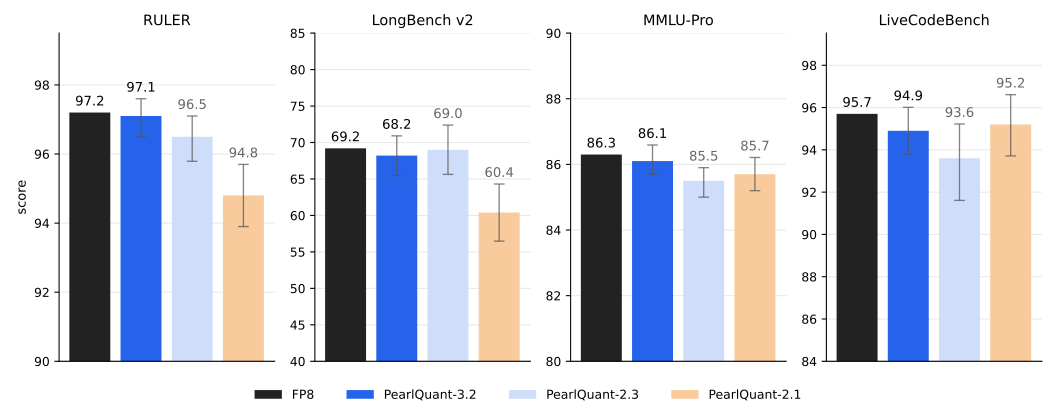
PearlQuant-3.2 shows no statistically significant difference from FP8 on any of the four benchmarks. The stress configuration PearlQuant-2.1 drops on the two long-context benchmarks.
Layer 3: the generated text
On MMLU-Pro and LiveCodeBench, even PearlQuant-2.1 loses less than a point. But a closer look at its reasoning can reveal subtle problems. For example, the model sometimes returns to the same passage repeatedly:
Wait, the text says: “One common strategy for rendering 2D Gaussians is to project the 2D Gaussian primitives onto the image space…” …
Wait, the text says: “One common strategy for rendering 2D Gaussians is to project the 2D Gaussian primitives onto the image space…”
The model behaves as if it cannot trust its memory of the text, so it reads it again. Since this is the symptom we found in the stress transcripts, we measure it directly: the number of times “Wait” appears per 1,000 words of reasoning. We also ask a blind judge whether the generated text got worse.
Blind self-judge. We compare only MMLU-Pro responses with the same final answer, to avoid bias from the judge inferring which answer is correct (even though it is not given the question). We show both reasoning texts, in random order, to GLM-5.3 itself (with an FP8 cache), without mentioning quantization, and ask whether one is worse and, if so, which one. We report how often it blames the compressed answer when it sees a difference (50% is chance). The results suggest that self-judging can be a useful check on quality: for any model, if the unquantized model can tell its quantized version apart, the damage is too large.
| FP8 | PearlQuant-3.2 | PearlQuant-2.3 | PearlQuant-2.1 | |
|---|---|---|---|---|
| “Wait” per 1,000 words, vs FP8 (LongBench v2 / MMLU-Pro / LiveCodeBench) | — | -1% / +2% / +3% | +10% / +28% / +13% | +77% / +106% / +48% |
| self-judge: quantized KV cache answer judged worse (800 MMLU-Pro questions) | 52.5%² | 53.2% | 52.7% | 69.7% |
Lower is better in both rows. For the self-judge, 50% is chance. Red marks the clear degradation.
² A second FP8 run judged against the first.
PearlQuant-2.1 says “Wait” twice as often as FP8 on MMLU-Pro, and the judge blames it 70% of the time (95% confidence interval: 66-73%). PearlQuant-3.2 is within a few percent of FP8 on “Wait”, and the judge is at chance, as for a second FP8 run.
Which configuration do we choose?
We base the decision on all three layers. PearlQuant-2.1 fails all of them. PearlQuant-2.3 may pass the judge, but shows slight degradation on benchmarks. It also shows more “Wait” in them: early signs of the damage that is obvious at 2.1. PearlQuant-3.2 shows none of these signs: no significant drop on any benchmark, a “Wait” rate within a few percent of FP8, and a judge at chance. We select PearlQuant-3.2 as the best trade-off between compression and quality.
Serving performance
So we showed that PearlQuant-3.2 preserves accuracy and text quality with a much smaller KV cache, but would it translate into faster serving? A quantizer can look excellent on paper, but slow decoding can erase its practical benefits. PearlQuant’s algorithm was designed specifically to enable fast KV cache decoding.
We served the model on one node of 8×B200 using vLLM with LMCache, eight-way data parallelism (DP=8) with expert parallelism and speculative decoding. We replay real Claude Code sessions from the AgentX dataset [12]. Only the KV cache quantization format changes between the runs. We compare PearlQuant with the two formats that vLLM supports natively, FP8 and NVFP4 (TurboQuant is not included as its available kernels do not support GLM-5.3’s DSA attention).
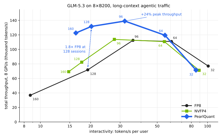
- At light load (32 sessions), FP8 is about 5% faster in requests per second. PearlQuant is on par with NVFP4, which has native hardware support on Blackwell. Decoding the lattice inside the kernel thus costs about as much as decoding a hardware-native format.
- As load grows, PearlQuant’s smaller cache reduces evictions and recomputation. Peak throughput is 24% higher than FP8's and 22% higher than NVFP4's. At 128 sessions, PearlQuant delivers 1.8× FP8's throughput, and the 90th-percentile time to first token is 7 seconds instead of 144.
Summary and outlook
We introduced PearlQuant, a higher-dimensional KV cache quantization method that combines high quality with fast decoding, demonstrating more efficient serving of GLM-5.3 under a realistic long-context workload. Future work will explore ways to shrink the KV cache further, including adaptive bit allocation across dimensions and time, and joint compression of multiple cache entries.
References
- [1]NVIDIA, Introducing NVFP4 for Efficient and Accurate Low-Precision Inference, NVIDIA Technical Blog, June 2025.
- [2]A. Zandieh, M. Daliri, M. Hadian, V. Mirrokni, TurboQuant: Online Vector Quantization with Near-optimal Distortion Rate, ICLR 2026. arXiv:2504.19874.
- [3]S. Savkin, E. Porat, O. Ordentlich, Y. Polyanskiy, NestQuant: Nested Lattice Quantization for Matrix Products and LLMs, ICML 2025. arXiv:2502.09720.
- [4]Wikipedia, E8 lattice.
- [5]T. M. Cover, J. A. Thomas, Elements of Information Theory, 2nd ed., Wiley, 2006, Chapter 10, “Rate Distortion Theory.” doi:10.1002/047174882X.ch10.
- [6]J. W. Rae, A. Potapenko, S. M. Jayakumar, T. P. Lillicrap, Compressive Transformers for Long-Range Sequence Modelling, ICLR 2020. arXiv:1911.05507.
- [7]H. He and Thinking Machines Lab, Defeating Nondeterminism in LLM Inference, Thinking Machines Lab: Connectionism, September 2025. doi:10.64434/tml.20250910.
- [8]C.-P. Hsieh et al., RULER: What's the Real Context Size of Your Long-Context Language Models?, COLM 2024. arXiv:2404.06654.
- [9]Y. Bai et al., LongBench v2: Towards Deeper Understanding and Reasoning on Realistic Long-context Multitasks, 2024. arXiv:2412.15204.
- [10]Y. Wang et al., MMLU-Pro: A More Robust and Challenging Multi-Task Language Understanding Benchmark, NeurIPS 2024, Datasets and Benchmarks Track. arXiv:2406.01574.
- [11]N. Jain et al., LiveCodeBench: Holistic and Contamination Free Evaluation of Large Language Models for Code, 2024. arXiv:2403.07974. Our evaluation: Easy+medium problems from November 2024 onward, with four runs per problem to reduce noise (564 items per arm).
- [12]SemiAnalysis, cc-traces-weka-062126, 2026. Claude Code session traces used in our serving evaluation with AIPerf 13.0. See also InferenceX AgentX: Methodology.